Why R?

• R is open source
• R has many statistical capabilities
• R can create custom data visualizations
• R has a large community of users

What is RStudio?

• RStudio is an integrated development environment (IDE) for R
• RStudio provides a user-friendly interface for coding
• RStudio Desktop is the most commonly used version of the software
• Posit (formerly known as RStudio) is the company that devloped and maintains RStudio

Exploring the IDE

Some key concepts

You will hear these terms often this week:

• Objects
• Variables
• Data Frames
• Functions
• Packages

Starting with the basics

• Arithmetic with R
• Objects and variable assignment
• Data types, incl.: character, numeric, logical, factors
• Data structures, incl.: vectors, matricies, data frames, lists

Our materials

All of our materials are available at github.com/NUMLDS/bootcamp-2025. Today, you will only need to work with two files, which are in the ZIP file linked at the top of the Github page.

Starting with the R3 session later this week, you will be working with a much wider set of files. You will also learn how to make a copy of the whole bootcamp-2025 repository using Git.

Arithmetic

At its most basic level, you can use R as a calculator. The basic operators are all what you would expect for addition (+), subtraction (-), multiplication (*), division (/), and exponentiation (^). You can use parentheses to indicate which operation should take place first.

You can save numbers or the results of operations as objects (whose names must start with a character) using the assignment operator <- or a single equal sign =. We sometimes call these objects variables. Look in the Environment to see what objects currently exist.

x <- 11*5
x

## [1] 55

Arithmetic: exercise

Open up the file R1-R2_exercises.R in RStudio.
Do the following tasks:

• Pick a number; save it as x
• Multiply x by 3
• Take the log of the above
• Subtract 4 from the above
• Square the above

Arithmetic: exercise

x <- 5
x*3

## [1] 15

log(x*3)

## [1] 2.70805

(log(x*3))-4

## [1] -1.29195

((log(x*3))-4)^2

## [1] 1.669134

Functions

Functions are called with functionName(parameters). Multiple paramters are comma-separated. Paramters can be named. For unnamed parameters, the order matters. R functions don’t change the objects passed to them (more on this later).

Let’s take a look at a simple function, log(), which takes the log of a number. You can access its help file by entering ?log in the console. Do so now. What does the function do? What are the arguments?

Functions

# Take the natural log of 10
log(10)

## [1] 2.302585

# Take the log of 10 with base-2
log(10, base=2)

## [1] 3.321928

# Store the result of log(10) as a variable
y <- log(10)

Data types

• numeric: real or decimal

  • integer: a specific type; most numbers are numeric instead

  • complex: ex: 2+5i

• character: "text data", denoted with quotes
  ('single quotes' and "double quotes" both work)

• logical: TRUE or FALSE
  (When coerced into numeric type, TRUE=1 and FALSE=0)

• Use class() on an object to check its type

Data types

x <- "some text"
x

## [1] "some text"

class(x)

## [1] "character"

x <- 5
x

## [1] 5

class(x)

## [1] "numeric"

Logical Operators

The basic logical operators in R are:

• == for “is equal”; ! for “is not”

• & for “and”; | for “or”

• < for “lesser than”; > for “more than”

A statement with logical operators will return a logical object TRUE or FALSE.

Logical Operators

5 > 4

## [1] TRUE

(5 > 4) & (4 < 5)

## [1] TRUE

(5 > 4) | (4 < 5)

## [1] TRUE

!(4 > 5)

## [1] TRUE

Logical Operators: exercise

• Check if 1 is bigger than 2
• Check if 1 + 1 is equal to 2
• Check if it is true that the strings “eat” and “drink” are not equal to each other
• Check if it is true that 1 is equal to 1 AND 1 is equal to 2
  (Hint: remember what the operators & and | do)
• Check if it is true that 1 is equal to 1 OR 1 is equal to 2

Logical Operators: exercise

1 > 2

## [1] FALSE

(1 + 1) == 2

## [1] TRUE

"eat" != 'drink'

## [1] TRUE

(1==1) & (1==2)

## [1] FALSE

(1==1) | (1==2)

## [1] TRUE

Packages

• Install the package ggplot2
  (You only need to do this the first time)
• Load the package ggplot2
• Open the help file for the dataset mpg
  
  
• Homework: Install and load the package tidyverse and open the help file for the function recode

Packages

install.packages("ggplot2")

library(ggplot2)

?mpg

Vectors

• Vectors store multiple values of a single data type (i.e. vectors are homogeneous)

• Create a vector using the c() function

• Arithmetic operators and many functions can apply to vectors (i.e. some functions are vectorized)

• Vectors can be indexed by:

  • element position (vec[1])
  • ‘slice’ position (vec[1:3])
  • condition (vec[vec>2]).

Vectors

vec <- c("yes", "no", "maybe")
vec <- c(1, 2, 3)

vec[1]

## [1] 1

vec[vec<3]

## [1] 1 2

vec*2

## [1] 2 4 6

log(vec)

## [1] 0.0000000 0.6931472 1.0986123

Vectors: exercise

Return to the exercise file and complete the following tasks:

• Run the code to generate variables x1 and x2
• Select the 3rd element in x1
• Select the elements of x1 that are less than 0
• Select the elements of x2 that are greater than 1
• Create x3 containing the first five elements of x2
• Select all but the third element of x1

Vectors: exercise

set.seed(1234) 
x1 <- rnorm(5)
x2 <- rnorm(20, mean=0.5)
x1[3]

## [1] 1.084441

x1[x1 < 0]

## [1] -1.207066 -2.345698

x2[x2 > 1]

## [1] 1.006056 1.459494 2.915835

x3 <- x2[1:5]
x1[-3]

## [1] -1.2070657  0.2774292 -2.3456977  0.4291247

Interlude: Missing Values

Real-world data often include missing values. In R, missing values are stored as NA. Vectors containing any data type can contain missing values. Functions deal with missing values differently, and sometimes require arguments to specify how to deal with missing values.

vec <- c(1, 8, NA, 7, 3)
mean(vec)

## [1] NA

mean(vec, na.rm=TRUE)

## [1] 4.75

Interlude: Missing Values

You can check if a vector contains missing values by the function is.na(). Since this returns a logical vector, you can use sum() or mean() on the result to count the number or proportion of TRUE values.

is.na(vec)

## [1] FALSE FALSE  TRUE FALSE FALSE

sum(is.na(vec))

## [1] 1

mean(is.na(vec))

## [1] 0.2

Factors

• Factors are a special type of vector that are useful for categorical variables
• Factors have a limited number of levels that the variable can take, set by the user
• For categorical variables with natural ordering between categories, we often want to use ordered factors
• Create factors with factor(), which includes an argument for levels =

Factors

fac <- factor(c("red", "yellow", "green", "green","green"))

class(fac)

## [1] "factor"

levels(fac)

## [1] "green"  "red"    "yellow"

Lists

• Lists are like vectors, but more complex.
• Lists are heterogenous: they can store single elements, vectors, or even lists.
• You can keep multi-dimensional and ragged data in R using lists.
• You can index an element in a list using double brackets: [[1]]. Single brackets will return the element as a list.

Lists

my_list <- list(42, "Hello world!",  c(1, 2, 3, 4, 5))

my_list[1]

## [[1]]
## [1] 42

class(my_list[1])

## [1] "list"

my_list[[1]]

## [1] 42

class(my_list[[1]])

## [1] "numeric"

Matrices

• Matrices in R are two-dimensional arrays.
• Matrices are homogeneous: all values of a matrix must be of the same data type.
• You can initialize a matrix using the matrix() function.
• Matrices are used sparingly in R, primarily for numerical calculations or explicit matrix manipulation.
• Matrices are indexed as follows: mat[row no, col no].

Matrices

my_matrix <- matrix(data = 1:6, nrow = 2, ncol = 3)
my_matrix

##      [,1] [,2] [,3]
## [1,]    1    3    5
## [2,]    2    4    6

my_matrix[1, 2]

## [1] 3

Data frames

• Data frames are the core data structure in R. A data frame is a list of named vectors with the same length.
• Data frames are heterogeneous: the vectors in a data frames can each be of a different data type.
• Columns are typically variables and rows are observations.
• You can make make data frames with data.frame(), or by combining vectors with cbind() or rbind().
• Data frames can be indexed in the same way as matrices: df[row no, col no].
• Data frames can also be indexed by using variable/column names: df$var or df[["var"]].

Data frames: exercise

• Load the example data frame using the code provided
• Identify the number of observations (rows), number of variables (columns), and names of variables using str()
• Select the variable mpg
• Select the 4th row
• Square the value of the cyl variable and store this as a new variable cylsq

Data frames: exercise

str(mtcars)

## 'data.frame':    32 obs. of  11 variables:
##  $ mpg : num  21 21 22.8 21.4 18.7 18.1 14.3 24.4 22.8 19.2 ...
##  $ cyl : num  6 6 4 6 8 6 8 4 4 6 ...
##  $ disp: num  160 160 108 258 360 ...
##  $ hp  : num  110 110 93 110 175 105 245 62 95 123 ...
##  $ drat: num  3.9 3.9 3.85 3.08 3.15 2.76 3.21 3.69 3.92 3.92 ...
##  $ wt  : num  2.62 2.88 2.32 3.21 3.44 ...
##  $ qsec: num  16.5 17 18.6 19.4 17 ...
##  $ vs  : num  0 0 1 1 0 1 0 1 1 1 ...
##  $ am  : num  1 1 1 0 0 0 0 0 0 0 ...
##  $ gear: num  4 4 4 3 3 3 3 4 4 4 ...
##  $ carb: num  4 4 1 1 2 1 4 2 2 4 ...

mtcars$mpg

mtcars[4,]

##                 mpg cyl disp  hp drat    wt  qsec vs am gear carb
## Hornet 4 Drive 21.4   6  258 110 3.08 3.215 19.44  1  0    3    1

mtcars$cylsq <- (mtcars$cyl)^2

Working directories

The working directory is the folder where R scripts and projects look for files by default.

You can go to the Files tab in the bottom right window in RStudio and find the directory you want. Then you can set it as a working directory with an option in the “More” menu. Or you can use the setwd() as follows:

setwd("/nfs/home/krn5889/R sessions")

Reading files: read.csv()

gapminder <- read.csv("data/gapminder5.csv", stringsAsFactors=FALSE)

gapminder <- read.csv(file = "data/gapminder5.csv",
                       sep = ",",
                       stringsAsFactors = FALSE)

Reading files: exercise

• Check your working directory with getwd().
• Import the gapminder data set using read.csv() and see what happens in the Environment tab.
• Take a look at the data using head() and View()
  
  After installing tidyverse:
• Load the readr package
• Use read_csv() to load the gapminder data. Read the message generated in the console.

Reading files: exercise

getwd()
head(gapminder5)
View(gapminder5)

library(readr)
gapminder <- read_csv("data/gapminder5.csv")

## Rows: 1704 Columns: 6
## ── Column specification ────────────────────────────────────────────────────────
## Delimiter: ","
## chr (2): country, continent
## dbl (4): year, pop, lifeExp, gdpPercap
## 
## ℹ Use `spec()` to retrieve the full column specification for this data.
## ℹ Specify the column types or set `show_col_types = FALSE` to quiet this message.

Reading files

• You can read files using RStudio’s interface through the “Files” tab
• You can also read files from the full local path or from URLs
• For other file types, use the packages haven (Stata, SAS, SPSS) or readxl (Excel)

Roadmap for the rest of the R sessions

• Today we will learn how to do basic data manipulation and data visualization in base R

• Most commonly, you will do these tasks using specialized packages such as tidyverse or data.table

• So why teach these skills in base R?

  • This helps you understand how R works
  • Many packages rely on how these tasks work in base R
  • Useful for simple tasks in workflows that otherwise don’t involve much manipulation or visualization

Exploring data frames

• You can view data frames in RStudio with View() and examine other characteristics with str(), dim(), names(), nrow(), and more.

• When run on a data frame, summary() returns summary statistics for all variables.

• mean(), median(), var(), sd(), and quantile() are useful functions for variables.

• Frequency tables are a simple and useful way to explore discrete/categorical variables in data frames

  • table() creates a frequency table of one or more variables
  • prop.table() can turn a frequency table into a proportion table

Exploring data frames: exercise

• Run summary() on the gapminder data
• Find the mean of the variable pop
• Create a frequency table of the variable year using table()
• Create a proportion table of the variable continent using prop.table()
  (Hint: check the help file for prop.table() to see what the input should be)

Exploring data frames: exercise

summary(gapminder)

##    country               year           pop             continent        
##  Length:1704        Min.   :1952   Min.   :6.001e+04   Length:1704       
##  Class :character   1st Qu.:1966   1st Qu.:2.794e+06   Class :character  
##  Mode  :character   Median :1980   Median :7.024e+06   Mode  :character  
##                     Mean   :1980   Mean   :2.960e+07                     
##                     3rd Qu.:1993   3rd Qu.:1.959e+07                     
##                     Max.   :2007   Max.   :1.319e+09                     
##     lifeExp        gdpPercap       
##  Min.   :23.60   Min.   :   241.2  
##  1st Qu.:48.20   1st Qu.:  1202.1  
##  Median :60.71   Median :  3531.8  
##  Mean   :59.47   Mean   :  7215.3  
##  3rd Qu.:70.85   3rd Qu.:  9325.5  
##  Max.   :82.60   Max.   :113523.1

Exploring data frames: exercise

mean(gapminder$pop)

## [1] 29601212

table(gapminder$year)

## 
## 1952 1957 1962 1967 1972 1977 1982 1987 1992 1997 2002 2007 
##  142  142  142  142  142  142  142  142  142  142  142  142

prop.table(table(gapminder$continent))

## 
##     Africa   Americas       Asia     Europe    Oceania 
## 0.36619718 0.17605634 0.23239437 0.21126761 0.01408451

Subsetting

• One of the benefits of R is that we can work with multiple data frames at the same time

• We will often want to subset a data frame, i.e. work with a portion of the data frame

• There are two common ways to subset a data frame in base R

  • Index the data frame: gapminder[gapminder$continent=="Asia",] (note the use of a logical statement and the comma)
  • Use the subset() function: subset(gapminder, subset=continent=="Asia")

Sorting

• The sort() function reorders elements, in ascending order by default.

  • You can flip the order by using the decreasing = TRUE argument.

• The order() function gives you the index positions in sorted order.

• sort() is useful for quickly viewing vectors; order() is useful for arranging data frames.

Subsetting and Sorting: exercise

• Create a new data frame called gapminder07 containing only those rows in the gapminder data where year is 2007
• Created a sorted frequency table of the variable continent in gapminder07
  (Hint: use table() and sort())
• Print out the population of Mexico in 2007
• Try the bonus question if you have time

Subsetting and Sorting: exercise

gapminder07 <- subset(gapminder, subset = year==2007)
sort(table(gapminder07$continent))

## 
##  Oceania Americas   Europe     Asia   Africa 
##        2       25       30       33       52

gapminder07$pop[gapminder07$country=="Mexico"]

## [1] 108700891

head(gapminder07[order(gapminder07$pop, decreasing=TRUE),])

## # A tibble: 6 × 6
##   country        year        pop continent lifeExp gdpPercap
##   <chr>         <dbl>      <dbl> <chr>       <dbl>     <dbl>
## 1 China          2007 1318683096 Asia         73.0     4959.
## 2 India          2007 1110396331 Asia         64.7     2452.
## 3 United States  2007  301139947 Americas     78.2    42952.
## 4 Indonesia      2007  223547000 Asia         70.6     3541.
## 5 Brazil         2007  190010647 Americas     72.4     9066.
## 6 Pakistan       2007  169270617 Asia         65.5     2606.

Adding and removing columns

When cleaning or wrangling datasets in RStudio, we will often want to create new variables.

Two ways to add a vector as a new variable in R:

gapminder$newvar <- newvar

gapminder <- cbind(gapminder, newvar)

Removing columns is easy too:

gapminder$newvar <- NULL

gapminder <- gapminder[-"newvar"]

Recoding variables

• A common task when cleaning/wrangling data is recoding variables.

• Think about what the recoded variable should look like & then decide on an approach.

  • Sometimes, a single function can accomplish the recoding task needed. The new vector can then be assigned to a new column in the data frame.
  • If no single function comes to mind, we can initialize a new variable in the data frame, and assign values using indexes and conditional statements.
  • More complex recoding tasks can be accomplished with other packages like dplyr, which you can preview in the lecture notes.

Recoding variables: exercise

Use the data frame gapminder07 throughout this exercise.

• Round the values of the variable lifeExp using round(), and store this as a new variable lifeExp_round
• Print out the new variable to see what it looks like
• Read through the code that creates the new variable lifeExp_over70 and try to understand what it does.
• Try to create a new variable lifeExp_highlow that has the value “High” when life expectancy is over the mean and the value “Low” when it is below the mean.

Recoding variables: exercise

gapminder07$lifeExp_round <- round(gapminder07$lifeExp)
head(gapminder07$lifeExp_round)

## [1] 44 76 72 43 75 81

Recoding variables: exercise

gapminder07$lifeExp_over70 <- NA  # Initialize a variable containing all "NA" values
gapminder07$lifeExp_over70[gapminder07$lifeExp>70] <- "Yes"
gapminder07$lifeExp_over70[gapminder07$lifeExp<70] <- "No"
table(gapminder07$lifeExp_over70)

## 
##  No Yes 
##  59  83

Recoding variables: exercise

gapminder07$lifeExp_highlow <- NA
gapminder07$lifeExp_highlow[gapminder07$lifeExp>mean(gapminder07$lifeExp)] <- "High"
gapminder07$lifeExp_highlow[gapminder07$lifeExp<mean(gapminder07$lifeExp)] <- "Low"
table(gapminder07$lifeExp_highlow)

## 
## High  Low 
##   85   57

Aggregating

• Notice that the observations (i.e. rows) in our data frame are grouped; specifically, each country is grouped into a continent.

• We are often interested in summary statistics by groups.

• The aggregate() function accomplishes this: aggregate(y ~ x, FUN = mean) gives the mean of vector y for each unique group in x.

  • mean can be replaced by other functions here, such as median.

• Try it! In the exercise file, find the mean of life expectancy in 2007 for each continent.

Aggregating: exercise

aggregate(gapminder07$lifeExp ~ gapminder07$continent, FUN = mean)

##   gapminder07$continent gapminder07$lifeExp
## 1                Africa            54.80604
## 2              Americas            73.60812
## 3                  Asia            70.72848
## 4                Europe            77.64860
## 5               Oceania            80.71950

aggregate(lifeExp ~ continent, data = gapminder07, FUN = mean)

##   continent  lifeExp
## 1    Africa 54.80604
## 2  Americas 73.60812
## 3      Asia 70.72848
## 4    Europe 77.64860
## 5   Oceania 80.71950

Statistics

• Here are some easy statistical analyses to conduct in R

  • Correlations: cor(); Covariance: cov()
  • T-tests: t.test(var1 ~ var2), where var2 is the grouping variable
  • Linear regression: lm(y ~ x1 + x2, data = df)

• You can store the results of these functions in objects, which is especially useful for statistical models with many components.

Statistics: exercise

Use gapminder07 for all the below exercises.

You’re using some new functions, so refer to help files whenever you get stuck.

• Calculate the correlation between lifeExp and gdpPercap.
• Use a t-test to evaluate the difference in gdpPercap between “high” and “low” life expectancy countries. Store the results as t1, and then print out t1.

Statistics: exercise

cor(gapminder07$lifeExp, gapminder07$gdpPercap)

## [1] 0.6786624

t1 <- t.test(gapminder07$gdpPercap~gapminder07$lifeExp_highlow)
t1 <- t.test(gdpPercap~lifeExp_highlow, data=gapminder07)
t1

## 
##  Welch Two Sample t-test
## 
## data:  gdpPercap by lifeExp_highlow
## t = 10.564, df = 95.704, p-value < 2.2e-16
## alternative hypothesis: true difference in means between group High and group Low is not equal to 0
## 95 percent confidence interval:
##  12674.02 18539.14
## sample estimates:
## mean in group High  mean in group Low 
##          17944.685           2338.104

Note that t1 is stored as a list. You can now call up the components of the t-test when you need them.

Statistics: exercise

• Conduct a linear regression using lm() which predicts lifeExp as a function of gdpPercap and pop. Store the results as reg1.

  • You can define all the variables using the df$var syntax, or you can just use variable names and identify the data frame in the data = argument.
  • Examples are shown at the bottom of the help file for lm()

• Print out reg1.

• Run summary() on reg1.

Statistics: exercise

reg1 <- lm(lifeExp ~ gdpPercap + pop, data = gapminder07)
reg1

## 
## Call:
## lm(formula = lifeExp ~ gdpPercap + pop, data = gapminder07)
## 
## Coefficients:
## (Intercept)    gdpPercap          pop  
##   5.921e+01    6.416e-04    7.001e-09

summary(reg1)

## 
## Call:
## lm(formula = lifeExp ~ gdpPercap + pop, data = gapminder07)
## 
## Residuals:
##     Min      1Q  Median      3Q     Max 
## -22.496  -6.119   1.899   7.018  13.383 
## 
## Coefficients:
##              Estimate Std. Error t value Pr(>|t|)    
## (Intercept) 5.921e+01  1.040e+00  56.906   <2e-16 ***
## gdpPercap   6.416e-04  5.818e-05  11.029   <2e-16 ***
## pop         7.001e-09  5.068e-09   1.381    0.169    
## ---
## Signif. codes:  0 '***' 0.001 '**' 0.01 '*' 0.05 '.' 0.1 ' ' 1
## 
## Residual standard error: 8.87 on 139 degrees of freedom
## Multiple R-squared:  0.4679, Adjusted R-squared:  0.4602 
## F-statistic: 61.11 on 2 and 139 DF,  p-value: < 2.2e-16

Writing a data file

• We will often want to save the data frames as data files after cleaning/wrangling/etc.

• You can use write.csv() from base R or write_csv() from readr to do this.

• Try it! Save the data frame gapminder07 in the same directory that gapminder5.csv is located.

  • If you use write.csv() , set the argument row.names = FALSE

  • If you use write_csv(), it does not include row names/numbers by default

Writing a data file: exercise

write.csv(gapminder07, file="data/gapminder07.csv", row.names=FALSE)
write_csv(gapminder07, file="data/gapminder07.csv")

Save R objects

• You can save all objects in your workspace using save.image() or by clicking the “Save” icon in the Environment tab.

  • You can load all objects back in using load.image() or opening the .RData file that is created.
  • You can save specific objects in an .RData file with the save() function.

• If your script file is well-written, you should be able to retrieve all your objects just by running your code again.

• If you have a project with code that takes a long time to run, I would recommend using project files.

Base R vs. ggplot2

• We will only cover visualization briefly today, using some functions included in base R. Data scientists generally use other packages for data visualization, especially ggplot2, which we will cover next Monday.

• So why learn data visualization in base R?

  • Some of the simple functions are useful ways to explore data while doing analysis.
  • The syntax of visualization in base R is often adopted by other packages.

Histograms

• Histograms are a useful way to examine the distribution of a single variable. The base R function for histograms is simple: hist().

• Try it! Create a histogram of the variable lifeExp in gapminder07.

  • When you’re done, look at the help file and try to re-create the histogram, this time with a title and axis labels.
  • Bonus: Change the breaks = argument from its default setting and see what happens.

Histograms: exercise

hist(gapminder07$lifeExp, 
     main="Distribution of life expectancy across countries in 2007", 
     xlab="Life expectancy", ylab="Frequency")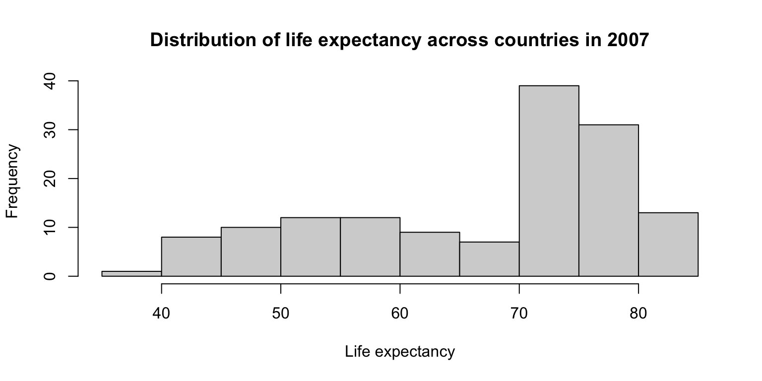

Scatterplots

• You can create a scatterplot by providing a formula containing two variables (i.e. y ~ x) to the plot() function in R.
• Titles and axis labels can be added in plot() similarly to hist().
• The function abline() can “layer” straight lines on top of a plot() output.

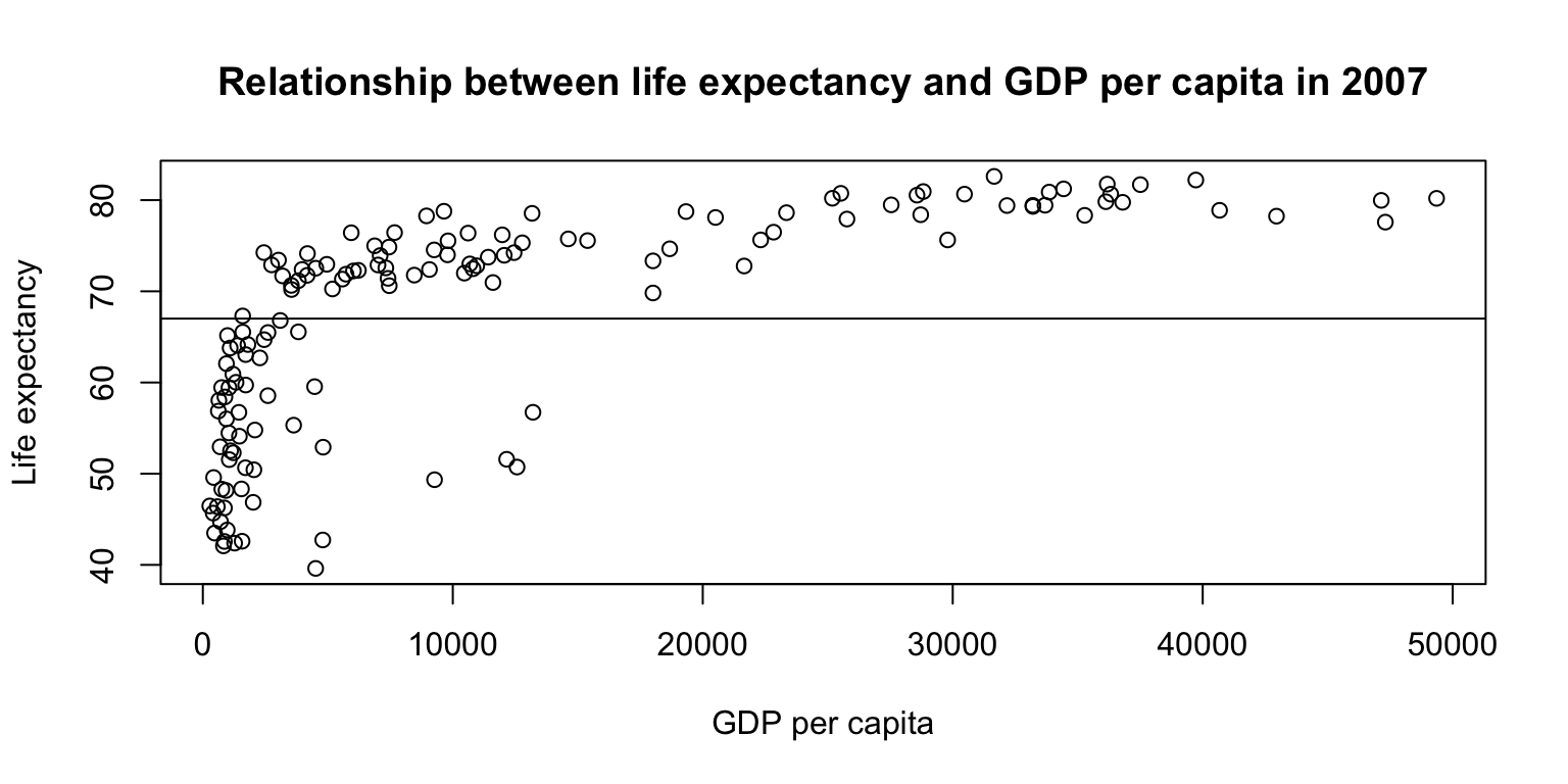
Scatterplots: exercise

• Create a scatterplot with lifeExp on the y-axis and gdpPercap on the x-axis.
• Add a title and axis labels.
• Bonus: Add a horizontal line indicating the mean of lifeExp onto the plot using abline().

Scatterplots: exercise

plot(gapminder07$lifeExp ~ gapminder07$gdpPercap)

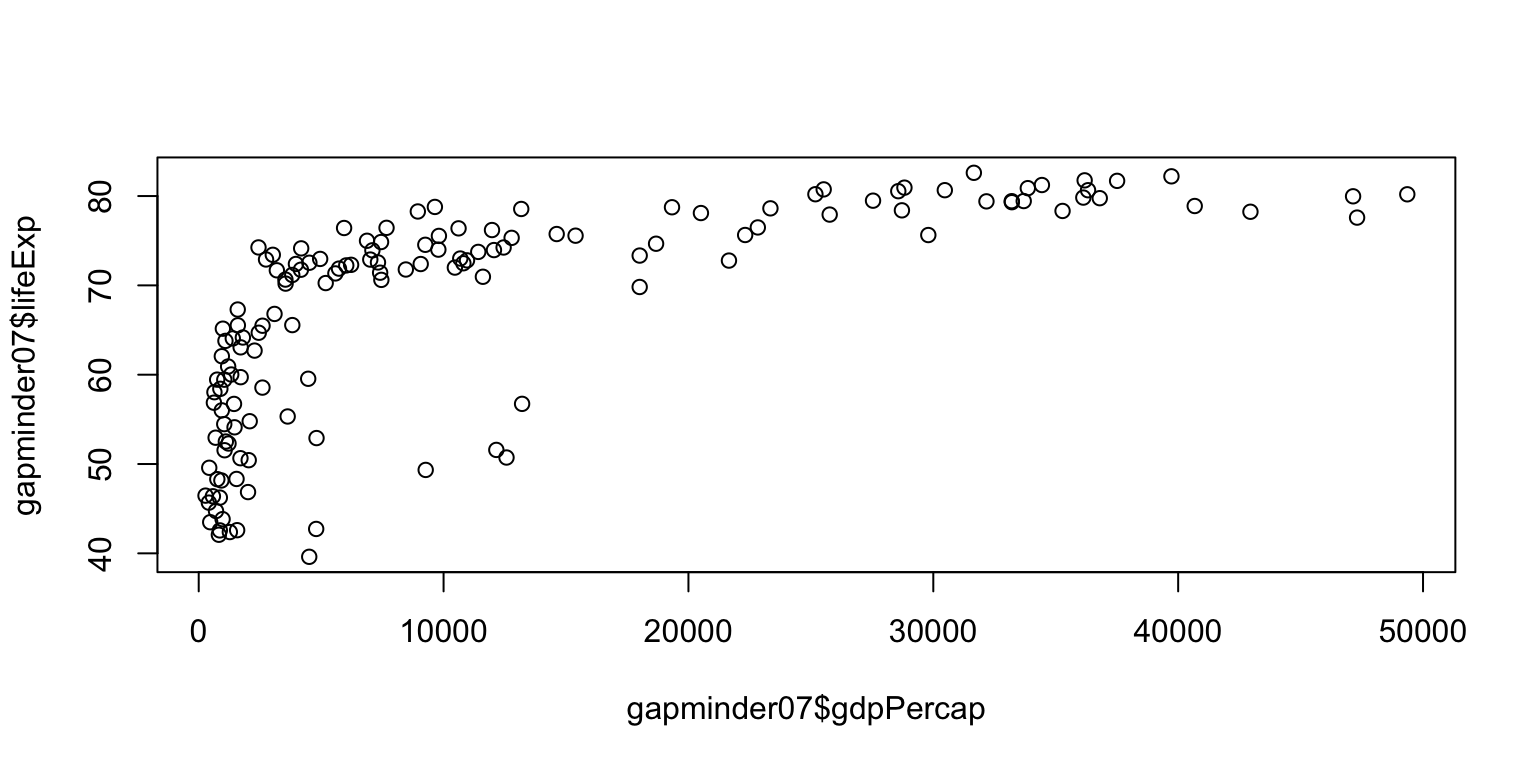
Scatterplots: exercise

plot(gapminder07$lifeExp ~ gapminder07$gdpPercap,
     main="Relationship between life expectancy and GDP per capita in 2007", 
     ylab="Life expectancy", xlab="GDP per capita")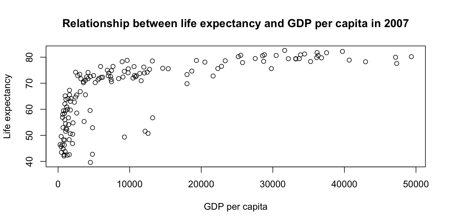

Scatterplots: exercise

plot(gapminder07$lifeExp ~ gapminder07$gdpPercap,
     main="Relationship between life expectancy and GDP per capita in 2007", 
     ylab="Life expectancy", xlab="GDP per capita")
abline(h = mean(gapminder07$lifeExp))